Plot a baseline hazard estimates from coxph_mpl_dc Object

Plot the baseline hazard with the confidence interval estimates

# S3 method for coxph_mpl_dc
plot(
  x,
  parameter = "theta",
  funtype = "hazard",
  xout,
  se = TRUE,
  ltys,
  cols,
  ...
)

Arguments

x	an object inheriting from class `coxph_mpl_dc`
parameter	the set of parameters of interest. Indicate `parameters="theta"` for the baseline hazard estimated by \(theta\) and `parameters="gamma"` for the baseline hazard estimated by \(gamma\)
funtype	the type of function for ploting, i.e. `funtype="hazard"` for baseline hazard, `funtype="cumhazard"` for baseline cumulative hazard and `funtype="survival"` for baseline survival function
xout	the time values for the baseline hazard plot
se	se=TRUE gives both the MPL baseline estimates and 95% confidence interval plots while se=FALSE gives only the MPL baseline estimate plot.
ltys	a line type vector with two components, the first component is the line type of the baseline hazard while the second component is the line type of the 95% confidence interval
cols	a colour vector with two components, the first component is the colour of the baseline hazard while the second component is the colour the 95% confidence interval
...	other arguments

Value

the baseline hazard plot

Details

When the input is of class coxph_mpl_dc and parameters=="theta", the baseline estimates base on \(\theta\) and xout (with the corresponding 95% confidence interval if se=TRUE ) are ploted. When the input is of class coxph_mpl_dc and parameters=="gamma", the baseline hazard estimates based on \(\gamma\) and xout (with the corresponding 95% confidence interval if se=TRUE ) are ploted.

References

Brodaty H, Connors M, Xu J, Woodward M, Ames D. (2014). "Predictors of institutionalization in dementia: a three year longitudinal study". Journal of Alzheimers Disease 40, 221-226.

Xu J, Ma J, Connors MH, Brodaty H. (2018). "Proportional hazard model estimation under dependent censoring using copulas and penalized likelihood". Statistics in Medicine 37, 2238–2251.

Author

Jing Xu, Jun Ma, Thomas Fung

Examples

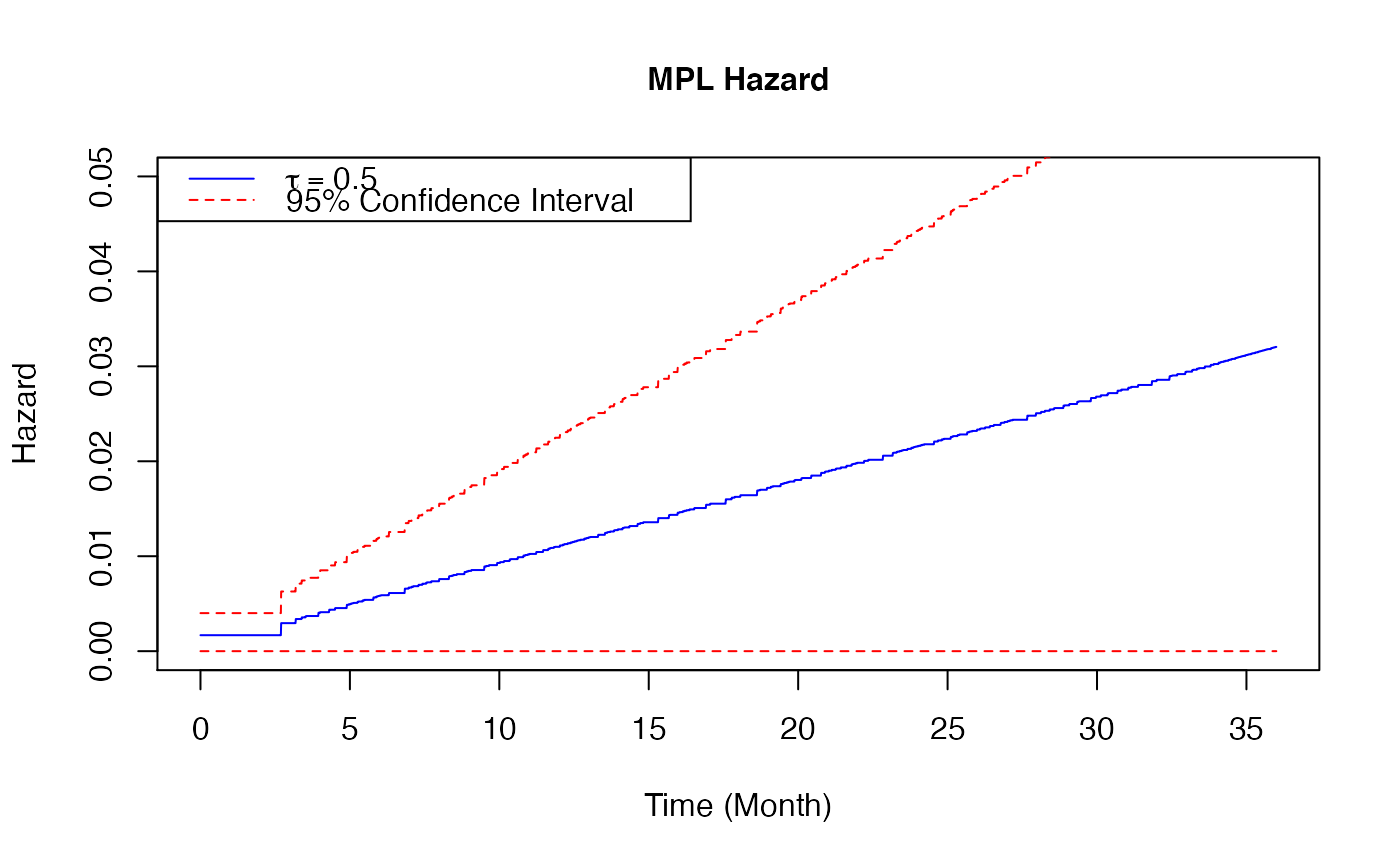
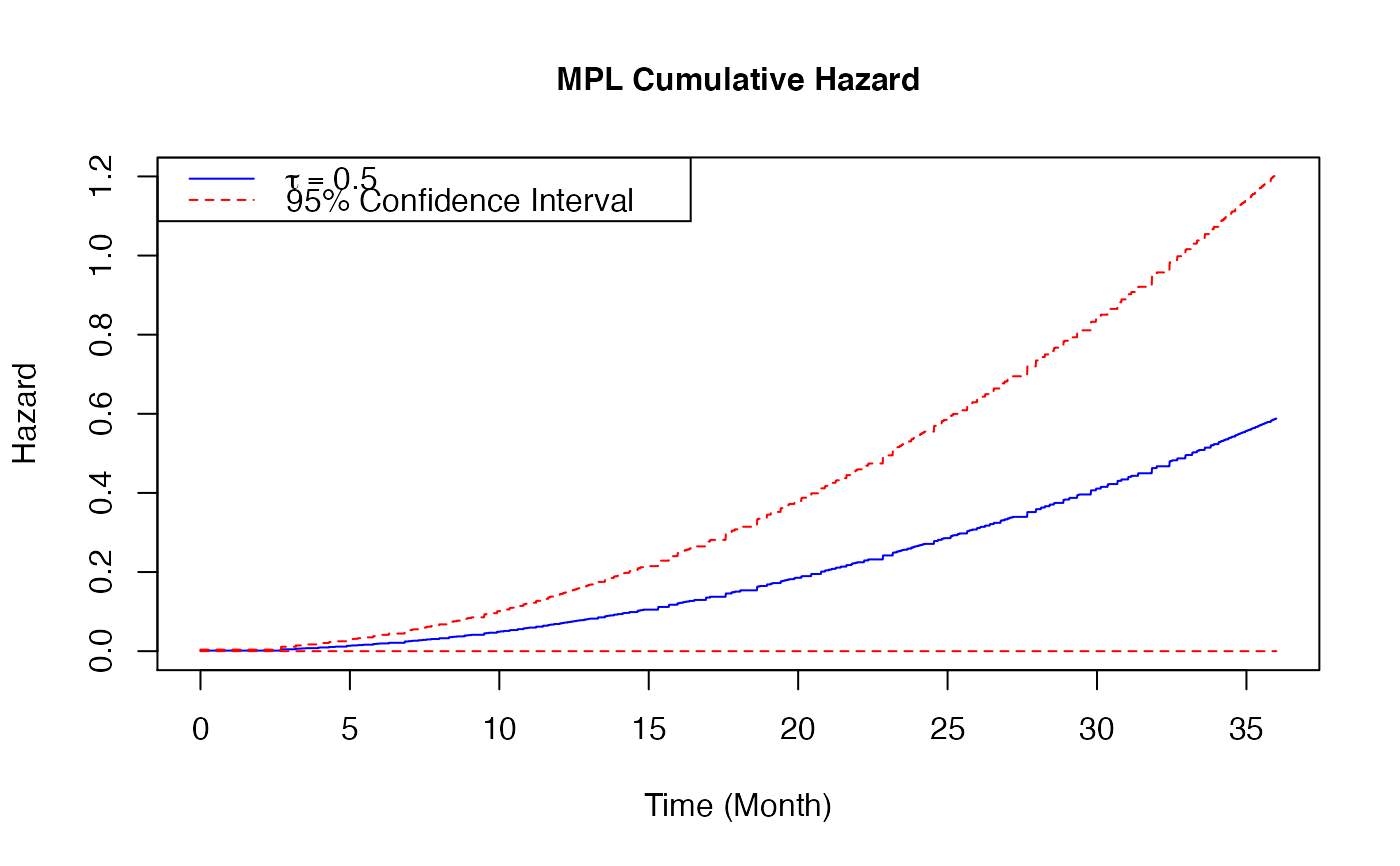
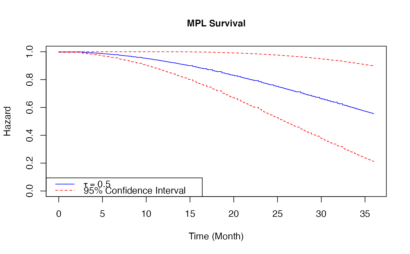
# \donttest{
 ##-- Copula types
 copula3 <- 'frank'

##-- A real example
##-- One dataset from Prospective Research in Memory Clinics (PRIME) study
##-- Refer to article Brodaty et al (2014),
##   the predictors of institutionalization of dementia patients over 3-year study period

data(PRIME)

surv<-as.matrix(PRIME[,1:3]) #time, event and dependent censoring indicators
cova<-as.matrix(PRIME[, -c(1:3)]) #covariates
colMeans(surv[,2:3])  #the proportions of event and dependent censoring
#>     Event    Depcen 
#> 0.2675815 0.2504288 

n<-dim(PRIME)[1];print(n)
#> [1] 583
p<-dim(PRIME)[2]-3;print(p)
#> [1] 15
names(PRIME)
#>  [1] "Time"           "Event"          "Depcen"         "Age"           
#>  [5] "Gender"         "HighEdu"        "Alzheimer"      "CDR_base"      
#>  [9] "MMSE_base"      "SMAF_base"      "ZBI_base"       "NPI_base"      
#> [13] "Benzon"         "Antiphsy"       "LivingAlone"    "MMSE_change_3m"
#> [17] "SMAF_change_3m" "NPI_change_3m" 

##--MPL estimate Cox proportional hazard model for institutionalization under medium positive
##--dependent censoring
control <- coxph_mpl_dc.control(ordSp = 4,
                                binCount = 200, tie = 'Yes',
                                tau = 0.5, copula = copula3,
                                pent = 'penalty_mspl', smpart = 'REML',
                                penc = 'penalty_mspl', smparc = 'REML',
                                cat.smpar = 'No' )

coxMPLests_tau <- coxph_mpl_dc(surv=surv, cova=cova, control=control, )

plot(x = coxMPLests_tau, parameter = "theta", funtype="hazard",
     xout = seq(0, 36, 0.01), se = TRUE,
     cols=c("blue", "red"), ltys=c(1, 2), type="l", lwd=1, cex=1, cex.axis=1, cex.lab=1,
     xlab="Time (Month)", ylab="Hazard",
     xlim=c(0, 36), ylim=c(0, 0.05)
     )
     title("MPL Hazard", cex.main=1)
     legend( 'topleft',legend = c( expression(tau==0.5), "95% Confidence Interval"),
     col = c("blue", "red"),
     lty = c(1, 2),
     cex = 1)

plot(x = coxMPLests_tau, parameter = "theta", funtype="cumhazard",
    xout = seq(0, 36, 0.01), se = TRUE,
    cols=c("blue", "red"), ltys=c(1, 2),
    type="l", lwd=1, cex=1, cex.axis=1, cex.lab=1,
    xlab="Time (Month)", ylab="Hazard",
    xlim=c(0, 36), ylim=c(0, 1.2)
)
title("MPL Cumulative Hazard", cex.main=1)
legend( 'topleft',
       legend = c( expression(tau==0.5), "95% Confidence Interval"),
       col = c("blue", "red"),
       lty = c(1, 2),
       cex = 1
)

plot(x = coxMPLests_tau, parameter = "theta", funtype="survival",
    xout = seq(0, 36, 0.01), se = TRUE,
    cols=c("blue", "red"), ltys=c(1, 2),
    type="l", lwd=1, cex=1, cex.axis=1, cex.lab=1,
    xlab="Time (Month)", ylab="Hazard",
    xlim=c(0, 36), ylim=c(0, 1)
)
title("MPL Survival", cex.main=1)
legend( 'bottomleft',
       legend = c( expression(tau==0.5), "95% Confidence Interval"),
       col = c("blue", "red"),
       lty = c(1, 2),
       cex = 1
)

# }